Notes: Multiview Geometry
Multiview Geometry
I’ve been learning about Multiview Geometry recently and the thing that hasn’t helped is starting from Hartley and Zisserman’s bible on the first go 😉.
Some things I’d wish I had gotten a stronger grasp on the coordinate systems and the homogeneous/ inhomogeneous representations of primitives.
As has been dealt with many-a-times, the camera matrix $\textbf{P}$ is simply a mapping of the world coordinate system into the camera coordinate system.
\[\mathbf{P} = \mathbf{K}[\mathbf{R}|\mathbf{t}]\]It first comprises of the extrinsics \([\mathbf{R} \vert \mathbf{t}]\), which is a rototranslation.
Additionally there are the camera intrinsics \(\mathbf{K}\), which first handles the focal-length induced scaling (due to similar triangles) and then shifts the coordinate system to positive image coordinates (origin at top left corner of image).
I found that coding and visualising the objects (using something like NumPy and Open3D for visualisation) also forced me to think about the coordinate systems and was beneficial for understanding.
Epipolar Geometry
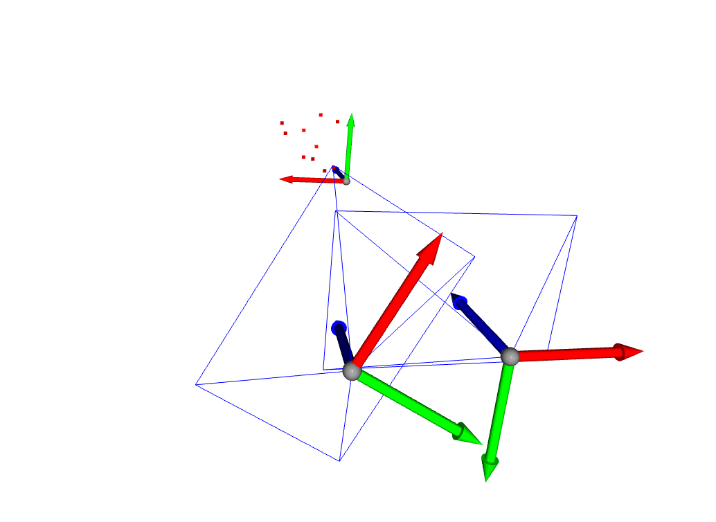 Two cameras
In this simulation, I generated several points, and then simulated the view of these points from the perspective of two pinhole cameras. We can find the Fundamental matrix of the two cameras using the image coordinates of the points in the two frames. After that, given the camera intrinsics, we can compute the essential matrix and subsequently decompose it to find the rototranslation from camera 1 to camera 2.
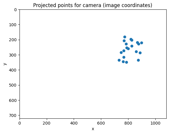 Result of forward projection into a single pinhole camera
This means that we have the relative pose of camera 2 to camera 1. By applying a triangulation operation, we are then able to back-project the locations of the original coordinates, up to a scale.
Code can be found here on GitHub.
Further resources
- Multiple View Geometry in Computer Vision, Second Edition
- Nice interactive visualisation on the action of the camera matrix
This is also the first article with mathjax :)