Backpropagation of the batch norm layer
Assignment 2 of Stanford’s CS231n took me a while to wrap my head round. These are some notes so that I remember.
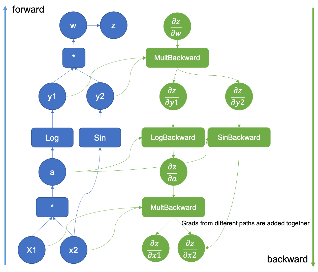
Backpropagation
A gradient estimation method using reverse mode differentiation!
In learning algorithms, the gradient we most often require is the gradient of the cost function with respect to the parameters, \(\nabla_W L(W)\) where \(W\) are the weights and $L$ is the scalar loss function.
Batch Norm
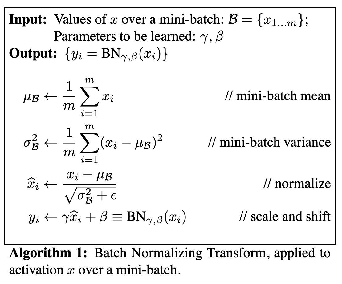 Algorithm from the original paper
Forward pass
# Elementwise statistics, average over batch
sample_mean = np.mean(x, axis=0)
sample_var = np.var(x, axis=0)
denom = np.sqrt(sample_var + eps)
# normalise
x_corrected = (x - sample_mean)/ denom #xhat
out = gamma * x_corrected + beta #yi

# Track the statistics of the mean and variance for test time
running_mean = momentum * running_mean + (1 - momentum) * sample_mean
running_var = momentum * running_var + (1 - momentum) * sample_var

cache = {'x_hat':x_corrected,
'mu':sample_mean,
'var':sample_var,
'denom':denom, 'gamma':gamma, 'beta':beta, 'x':x
}
Method 1: Computational Graph
We trace the computational graph backwards step by step. This was explained here quite well!
dgammax = dout # dL/d(gamma*x)
dgamma = np.sum(dgammax * xhat, axis=0) #dL/dgamma
dxhat = dgammax * gamma # dL/dxhat
dbeta = np.sum(dout, axis=0) # dL/dbeta

dnom_1 = dxhat * (1/denom) #dL/d(x-mu)
ddenom = np.sum(dxhat * - nom/ denom**2, axis=0) # dL/d(sqrt(var+eps))
dvar = ddenom * 0.5/denom #dL/dvar

dnom_2 = dvar * 2 * x / N #dL/d(x-mu)
dnom = dnom_1 + dnom_2 #dL/dnom
dmu = -1 *  np.sum(dnom, axis=0) #dL/dmu
dx_1 = dmu * np.ones((N,D)) / N
dx_2 = dnom
dx = dx_1 + dx_2
Method 2: Differentiation from first principles
This is already well explained in this blogpost, but I’d just like to add some more intuition.
Example 1: Say we have a zero-centering/ mean subtraction operation using statistics derived from a batch. So \(y = x - \mu\). We know that \(x\) and \(y\) have the same size \(x,y \in \mathbb{R}^{(N\times D)}\) where $N$ is the batch size and \(D\) is the number of dimensions in your training example. If we write all the entries of matrix \(y\) out this will be
\[y_{kl} = x_{kl}- \frac{1}{N}\sum_{i}^{n}x_{il}\]Equation 1: mean shift operation.
more verbosely, using the Kronecker delta notation, which explicitly tells you the rules of the transition from \(x\) to \(y\), and we label the indices \(i,j\) and \(k,l\) differently for matrices \(x\) and \(y\) for clarity.
\[y_{kl} =x_{ij}\delta_{ik}\delta_{jl} - \frac{1}{N}\sum_{i}^{n}x_{ij}\delta_{jl}\]Equation 1: matrix entry view of batch mean subtraction. This tells you how each element in the training batch will affect the output.
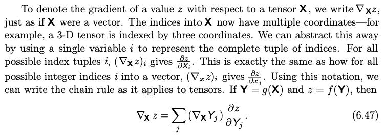
Say we already measured how much \(y\) impacts the scalar loss \(L\). In other words, we know the upstream derivative, a 2D matrix \(\frac{dL}{dy_{kl}}\), which is how much the loss \(L\) changes by as each entry in \(y_{kl}\) changes. However, we want to use backpropagation to compute the loss with respect to $x$. We use the chain rule and sum over the indices in \(y\).
\[\frac{dL}{dx_{ij}} = \sum_{kl}\frac{dL}{dy_{kl}} \frac{dy_{kl}}{dx_{ij}}\]The complicated thing here is that \(x\) and \(y\) are matrices/ tensors. This is explained away in the deep learning book.
The terms
- \(\frac{dL}{dy_{kl}}\) as explained, a 2D matrix
- \(\frac{dy_{kl}}{dx_{ij}}\) is called a Jacobian matrix here (2x2 = 4D), which explains how much each element in matrix \(y\) changes as each element in matrix \(x\) changes.
We write down the Jacobian computing the derivative of Eq. 1
\[\frac{dy_{kl}}{d x_{ij}} = \delta_{ik}\delta_{jl}-\frac{1}{N}\delta_{jl}\]Eq. 2: Jacobian of the mean shift operation
Now we compute the loss by subtituting Eq.2 into the sum
\[\frac{d L}{d x_{ij}} = \frac{dL}{d x_{ij}} - \frac{1}{N} \sum_k \frac{dL}{dy_{kj}}\]Eq. 3 Backpropagated gradient wrt $x$ of the loss function.
See that \(\delta_{jl}\) is in both terms, which means that the channels are taken to be independent in the mean shift, as expected :)
Some additional interpretation: Consider the first term in Eq. 1, as \(x\) changes, the same amount is changed in \(y\). The second term is a bit trickier. Changing one entry of \(x\) affects the batch mean, and so affects the ‘zero point’ of the entire batch, affecting every entry in \(y\)! But by how much? In fact a change \(dx\) in \(x\) will result in the outcome of each entry of \(y\) to change by \(dy = 1/N\). However, we ultimately care about the effect on the loss, which is why we are summing over indices \(kl\). The insight here is that the term \(\mu\) means that each row of \(\frac{dL}{dx_{ij}}\) will have contributed to all \(y_{kl}\).
Example 2: Say we have a variance operation. So \(Y = \frac{1}{N}\sum_i(X - \mu)^2\).
\[\frac{\partial \sigma^2_l}{\partial x_{ij}} = \frac{2}{N} (x_{ij} - \mu_l)\delta_{jl}\]Interpretation
- each element \(x_{ij}\) only affects the variance in the dimension that its relevant in, due to the Kronecker delta
- a change in the mean itself will not affect the variance if the values’ excess from the mean stays the same (think of the variance being the same when the entries are all shifted by a constant amount)
Full Solution to Batch Norm:
\[\frac{\partial L}{\partial x_{ij}} = \sum _{kl} \frac{\partial L}{\partial y_{kl}}\frac{\partial y_{kl}}{\partial x_{ij}}\]Use the product rule
\[\frac{\partial y_{kl}}{\partial x_{ij}} = \gamma_l \bigg [ \frac{\partial (x_{kl} - \mu_l)}{\partial x_{ij}}\cdot (\sigma^2_{l} + \epsilon)^{-\frac{1}{2}} + \frac{\partial (\sigma^2_{l} + \epsilon)^{-\frac{1}{2}} }{\partial x_{ij}}\cdot (x_{kl} - \mu_l) \bigg] \\ = \gamma_l \bigg[ (\delta_{ik}\delta_{jl} - \frac{1}{N}\delta_{jl}) \cdot(\sigma^2_{l} + \epsilon)^{-\frac{1}{2}} -\frac{1}{2} (\sigma^2_{l} + \epsilon)^{-\frac{3}{2}} \frac{2}{N} (x_{ij} - \mu_l)\delta_{jl}\cdot (x_{kl} - \mu_l) \bigg]\]Now we sum over indices \(k,l\)
\(\frac{\partial L}{\partial x_{ij}}\)
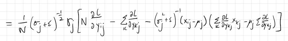
In code, this is
N, D = dout.shape
gamma = cache['gamma']
denom = cache['denom'] # sqrt(var + eps)
mu = cache['mu']
var = cache['var']
x = cache['x']
nom = x-mu
xhat = cache['x_hat'] # (x-mu)/denom

dgamma = np.sum(dout * xhat, axis=0) #dL/dgamma
dbeta = np.sum(dout, axis=0) # dL/dbeta

sum_dout_batch = np.sum(dout, axis=0) #sum_k dL/dout_kj
sum_doutnom_batch = np.sum(dout * nom, axis=0) #sum_k dL/dout_kj * xkj
dx = (1 / N) * gamma * denom **(-1) * (N * dout - sum_dout_batch - nom * denom**(-2) * sum_doutnom_batch)
which leads to a 1.6x speedup roughly.
Side notes
Kronecker delta
Physicists here will be reminded of their classes in general relativity (tensors), atomic physics (dipole matrix transition elements).
Differences in resources
The deep Learning book draws nodes as intermediary variables
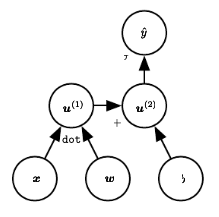
CS231n draws nodes as operations and treat nodes as ‘gates.’
The PyTorch docs illustrate both albeit in different shapes.
Additional notes on backprop
- https://colah.github.io/posts/2015-08-Backprop/ (Good for understanding Computational graphs and why backprop matters)
- Deep Learning book (Mathsy, as usual, good for a second pass once you’ve understood the material)